Data analysis case study with Hotel prices dataset. The detailed code and output(s) is on Github at below URL:-
https://github.com/srichallla/Analyzing_Hotels_Dataset/blob/master/HotelPrices_eda.ipynb
Lets first load the data and understand the features:-
RangeIndex: 221069 entries, 0 to 221068 Data columns (total 21 columns):
room_id 221069 non-null int64
host_id 221067 non-null float64
room_type 221055 non-null object
borough 0 non-null float64
neighborhood 221069 non-null object
reviews 221069 non-null int64
overall_satisfaction 198025 non-null float64
accommodates 219750 non-null float64
bedrooms 220938 non-null float64
price 221057 non-null float64
minstay 63969 non-null float64
latitude 221069 non-null float64
longitude 221069 non-null float64
last_modified 221069 non-null object
date 221069 non-null object
survey_id 70756 non-null float64
country 0 non-null float64
city 70756 non-null object
bathrooms 0 non-null float64
name 70588 non-null object
location 70756 non-null object
dtypes: float64(12), int64(2), object(7)
We don't have a business objective for this dataset. But, before performing exploratory data analysis, its good to define one. So here are some possible business objectives I could think of, by looking at the dataset and its features:-
1) Predict the hotel prices. it’s a supervised learning regression problem.
2) We can also classify prices as high, medium, low which make the objective as a supervised learning classification problem.
3) We can perform hotel segmentation using clustering, to find hidden patterns or meaningful clusters.
For the current analysis, my business objective would be to predict hotel prices.
Looking at the output of df.info(), we can infer:-
a) borough, country, and bathrooms features are all nulls, and hence can be dropped.
b) host_id, room_type, overall_satisfaction, accommodates, bedrooms, and price has 2,14,23044,1319,131 and 12 missing values respectively.
c) minstay has 157100 (more than 70%) missing values, hence we will not include it in our analysis.
d) survey_id has 150313 (more than 65%) missing values, we will drop it too.
e) city too has more than 65% missing values. Also it has only two unique values:- df.city.unique():[nan, 'Amsterdam']. So wi will drop it too.
f) name, and location has 150481 (68%), and 150313(67%) missing values. So will drop these.
g) Finally, I will also drop the "last_modified" feature from the analysis, as I feel it's not significant for analyzing our business objective of predicting hotel prices.
Just by looking at the summary of features. We were able to drop unwanted features. So we now
have 221069 rows and 12 columns in the dataset.
We will be merging the "room_id" and "host_id" and create a new feature "hotel_id". And then drop
those 2 features. Although it's better to concatenate these two features. Here I am going to add them up.
Let's plot some Boxplots to gain insights into some of the features

Looking at box plots above, we can notice significant outliers. It's good to understand if these are indeed outliers, if so, what caused these outliers, and finally how to deal with them.
Let's look at "bedrooms":-
df.bedrooms.unique()
array([ 1., 2., 3., nan, 4., 0., 5., 10., 7., 9., 6.,
8.])
Looking at above values, I feel individual house can have 10 bedrooms. And some rent just cabins, so 0 bedrooms are possible.
So I don't think these are outliers and hence we leave them as is.
Let's look at "accommodates"-
array([ 2., 4., 6., 3., 1., 5., 8., 7., 16., 12., 14.,
9., 10., 13., 15., 11., nan, 17.])
I think independent rented houses can accommodate 17. So we leave them as is.
Now let's look at some "Price" statistics:-
* Let's make an assumption that all "prices" in the dataset are per night in "Euros".
* With that assumption we can see that the cheapest hotel price is "10 Euros" and the costliest one is "9916 Euros" for one night.
Lets group by "neighborhood" and see if these outliers are specific to one neighborhood. As can be seen in below boxplot(s), there are outliers across many neighborhoods. And "9916 euros" per night seems to be too much. Also "10 euros" per night seems unreasonable to me. So let's remove these outliers from "price".

Also using R when I plot "latitude" and "longitude" on a map (see below). By looking at data points on the map, and also by verifying that "location" for all data points contains "Amsterdam", we can conclude that they all belong to one city and hence no outliers as far as location is concerned.
So we will drop "latitude", "longitude" from our dataset to reduce redundancy with "neighborhood" feature.


R script snippet for above map plottings
There are various ways to treat the outliers, but one approach that statisticians follow is based on Inter-Quartile range(IQR). Where IQR = 75% - 25% (3rd-1st quartile),we get from df.price.describe() . Anything that's above and below 1.5*IQR can be removed. And that's what we are going to do here.
Note: In real time whenever we are making assumptions or performing data transformations like treating outliers etc. on data, its always advisable to discuss with the domain expert.
Below diagram depicts price boxplot after removing outliers.

Let's see if a relationship exists between Price and neighborhood. Let's get the "mean" price by neighborhood and plot a barchart.
Here I am plotting top 15 of 23 neighborhoods to prevent cluttering.
Looks like some neighborhood hotel rates are costlier than others, see below barchart.

More often than not we need to look at multiple types of visulizations, to find patterns and gain insights.
So let's plot a scatterplot for price and neighborhood. But since scatterplot cannot work on text/string data for "neighborhood" let's map it to some integer values, and then plot it.
Lets create a new column 'neighborhood_num' with the mappings. We may later drop "neighborhood".

By looking at the above plot. Observe the datapoint(s) are clustered as vertical lines in the scatter plot, this is because each belongs to one neighbourhood. The regression line is going up which indicates a positive correlation between neighborhood and price. But to confirm let's also look at line plot.

Looks like there is mostly an upward trend in price and neighborhood (neighborhood_num). Will look at correlation scores a little later. Let's get into time series analysis.
There's a "date" column. Generally, Hotel prices are higher during weekends. We will create a new column "day_of_week" from "date" column.


https://github.com/srichallla/Analyzing_Hotels_Dataset/blob/master/HotelPrices_eda.ipynb
Lets first load the data and understand the features:-
df = pd.read_csv("bookings.csv",encoding='latin1')
df.info()
RangeIndex: 221069 entries, 0 to 221068 Data columns (total 21 columns):
room_id 221069 non-null int64
host_id 221067 non-null float64
room_type 221055 non-null object
borough 0 non-null float64
neighborhood 221069 non-null object
reviews 221069 non-null int64
overall_satisfaction 198025 non-null float64
accommodates 219750 non-null float64
bedrooms 220938 non-null float64
price 221057 non-null float64
minstay 63969 non-null float64
latitude 221069 non-null float64
longitude 221069 non-null float64
last_modified 221069 non-null object
date 221069 non-null object
survey_id 70756 non-null float64
country 0 non-null float64
city 70756 non-null object
bathrooms 0 non-null float64
name 70588 non-null object
location 70756 non-null object
dtypes: float64(12), int64(2), object(7)
We don't have a business objective for this dataset. But, before performing exploratory data analysis, its good to define one. So here are some possible business objectives I could think of, by looking at the dataset and its features:-
1) Predict the hotel prices. it’s a supervised learning regression problem.
2) We can also classify prices as high, medium, low which make the objective as a supervised learning classification problem.
3) We can perform hotel segmentation using clustering, to find hidden patterns or meaningful clusters.
For the current analysis, my business objective would be to predict hotel prices.
Looking at the output of df.info(), we can infer:-
a) borough, country, and bathrooms features are all nulls, and hence can be dropped.
b) host_id, room_type, overall_satisfaction, accommodates, bedrooms, and price has 2,14,23044,1319,131 and 12 missing values respectively.
c) minstay has 157100 (more than 70%) missing values, hence we will not include it in our analysis.
d) survey_id has 150313 (more than 65%) missing values, we will drop it too.
e) city too has more than 65% missing values. Also it has only two unique values:- df.city.unique():[nan, 'Amsterdam']. So wi will drop it too.
f) name, and location has 150481 (68%), and 150313(67%) missing values. So will drop these.
g) Finally, I will also drop the "last_modified" feature from the analysis, as I feel it's not significant for analyzing our business objective of predicting hotel prices.
Just by looking at the summary of features. We were able to drop unwanted features. So we now
have 221069 rows and 12 columns in the dataset.
We will be merging the "room_id" and "host_id" and create a new feature "hotel_id". And then drop
those 2 features. Although it's better to concatenate these two features. Here I am going to add them up.
df['hotel_id'] = df['room_id'] + df['host_id']
Let's plot some Boxplots to gain insights into some of the features

Looking at box plots above, we can notice significant outliers. It's good to understand if these are indeed outliers, if so, what caused these outliers, and finally how to deal with them.
Let's look at "bedrooms":-
df.bedrooms.unique()
array([ 1., 2., 3., nan, 4., 0., 5., 10., 7., 9., 6.,
8.])
Looking at above values, I feel individual house can have 10 bedrooms. And some rent just cabins, so 0 bedrooms are possible.
So I don't think these are outliers and hence we leave them as is.
Let's look at "accommodates"-
array([ 2., 4., 6., 3., 1., 5., 8., 7., 16., 12., 14.,
9., 10., 13., 15., 11., nan, 17.])
I think independent rented houses can accommodate 17. So we leave them as is.
Now let's look at some "Price" statistics:-
* Let's make an assumption that all "prices" in the dataset are per night in "Euros".
* With that assumption we can see that the cheapest hotel price is "10 Euros" and the costliest one is "9916 Euros" for one night.
Lets group by "neighborhood" and see if these outliers are specific to one neighborhood. As can be seen in below boxplot(s), there are outliers across many neighborhoods. And "9916 euros" per night seems to be too much. Also "10 euros" per night seems unreasonable to me. So let's remove these outliers from "price".

Also using R when I plot "latitude" and "longitude" on a map (see below). By looking at data points on the map, and also by verifying that "location" for all data points contains "Amsterdam", we can conclude that they all belong to one city and hence no outliers as far as location is concerned.
So we will drop "latitude", "longitude" from our dataset to reduce redundancy with "neighborhood" feature.


R script snippet for above map plottings
# Get the location with detailed address from Latitude and Longitude
result <- do.call(rbind,
                  lapply(1:nrow(df),
                         function(i)revgeocode(as.numeric(df[i,6:5]))))
df <- cbind(df,result)

#Now let’s plot this same data on an image from Google Maps using R's ggmap
AmsterdamMap<-qmap("amsterdam", zoom = 11)

"AmsterdamMap+                                        ##This plots the Amsterdam Map
geom_point(aes(x = longitude, y = latitude), data = df) "   ##This adds the points to it
There are various ways to treat the outliers, but one approach that statisticians follow is based on Inter-Quartile range(IQR). Where IQR = 75% - 25% (3rd-1st quartile),we get from df.price.describe() . Anything that's above and below 1.5*IQR can be removed. And that's what we are going to do here.
Note: In real time whenever we are making assumptions or performing data transformations like treating outliers etc. on data, its always advisable to discuss with the domain expert.
Below diagram depicts price boxplot after removing outliers.

Let's see if a relationship exists between Price and neighborhood. Let's get the "mean" price by neighborhood and plot a barchart.
Here I am plotting top 15 of 23 neighborhoods to prevent cluttering.
Looks like some neighborhood hotel rates are costlier than others, see below barchart.

More often than not we need to look at multiple types of visulizations, to find patterns and gain insights.
So let's plot a scatterplot for price and neighborhood. But since scatterplot cannot work on text/string data for "neighborhood" let's map it to some integer values, and then plot it.
Lets create a new column 'neighborhood_num' with the mappings. We may later drop "neighborhood".

By looking at the above plot. Observe the datapoint(s) are clustered as vertical lines in the scatter plot, this is because each belongs to one neighbourhood. The regression line is going up which indicates a positive correlation between neighborhood and price. But to confirm let's also look at line plot.

Looks like there is mostly an upward trend in price and neighborhood (neighborhood_num). Will look at correlation scores a little later. Let's get into time series analysis.
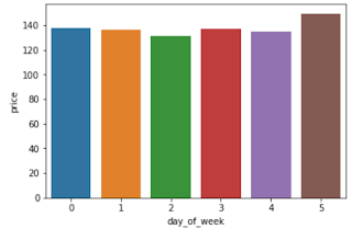
There's a "date" column. Generally, Hotel prices are higher during weekends. We will create a new column "day_of_week" from "date" column.
In the below barchart, during weekends, on Saturdays (day_of_week=5) average Hotel prices are high. There are no samples for Sunday in this dataset, strange!!!. In real time we need to check with domain expert(s) and/or other teams which are responsible to maintain data, like DB team.

Let's look at correlation heat map.

You can see that there's a positive correlation of 0.29 between price and neighborhood (neighborhood_num). So we are right.
But currently, we are dealing with over 200000 samples.
Note: Sometimes its enough to do analysis on a subset of the whole population. Let's see if above correlations between price, neighborhood (neighborhood_num) and other variables hold good for a subset of samples.
As we see that most of the hotels in a given neighbourhood have similar per night price. Let's find the sum of reviews, mean of overall_satisfaction, price and merge the original dataframe with a respective sum, mean values (Code is in accompanying Jupyter notebook).
Let's see if above correlations hold good for the subset of whole Hotels population.

We can see above that most of the correlations hold good for the subset of Hotel samples. So we can work with the subset from now on. Because working with a subset of samples saves training time and storage issues.
From the above correlations heatmap we can find:-
a) bedrooms and accommodates has a high positive correlation of 0.62, so we can consider only one of these two for predicting prices. And it's better to go with "accommodates", bcz it has a higher correlation of 0.45 with price.
b) Price and neighborhood (neighborhood_num) has a positive correlation of 0.31
Lets see if "room_type" has any relationship with Price, which is our target or dependent variable.

Looking at above barchart its clearly visible that there's a positive correlation between room_type and price. To find its correlation score we need to convert "room_type" from text/string to numeric.

As we can see above room_type (roomtype_num) and price has a positive correlation.
After type casting price from float to int and filtering out nulls, price distribution can be seen below.

In the price distribution above, mean is greater than the median, so the distribution is right-skewed. I am going to end my analysis here.
If anyone has a suggestion to view in a different dimension or another kind of plot(s) to gain more insights, please feel free to comment below.